Preamble
At the end of the spring of 2025, I started using some CAD software, preferably FOSS, because I wanted to design some furniture for myself.
I didn’t find anything that really clicked for me at the time.
While wondering I could make my own (as one do, you know), I made some intriguing discoveries1 2.
From this initial frustration and piqued curiosity, emerged a drive to write a simple CAD software:
fsolid.
It’s merely a prototype at this point, never was simple, and served more as a learning experience than a CAD software.
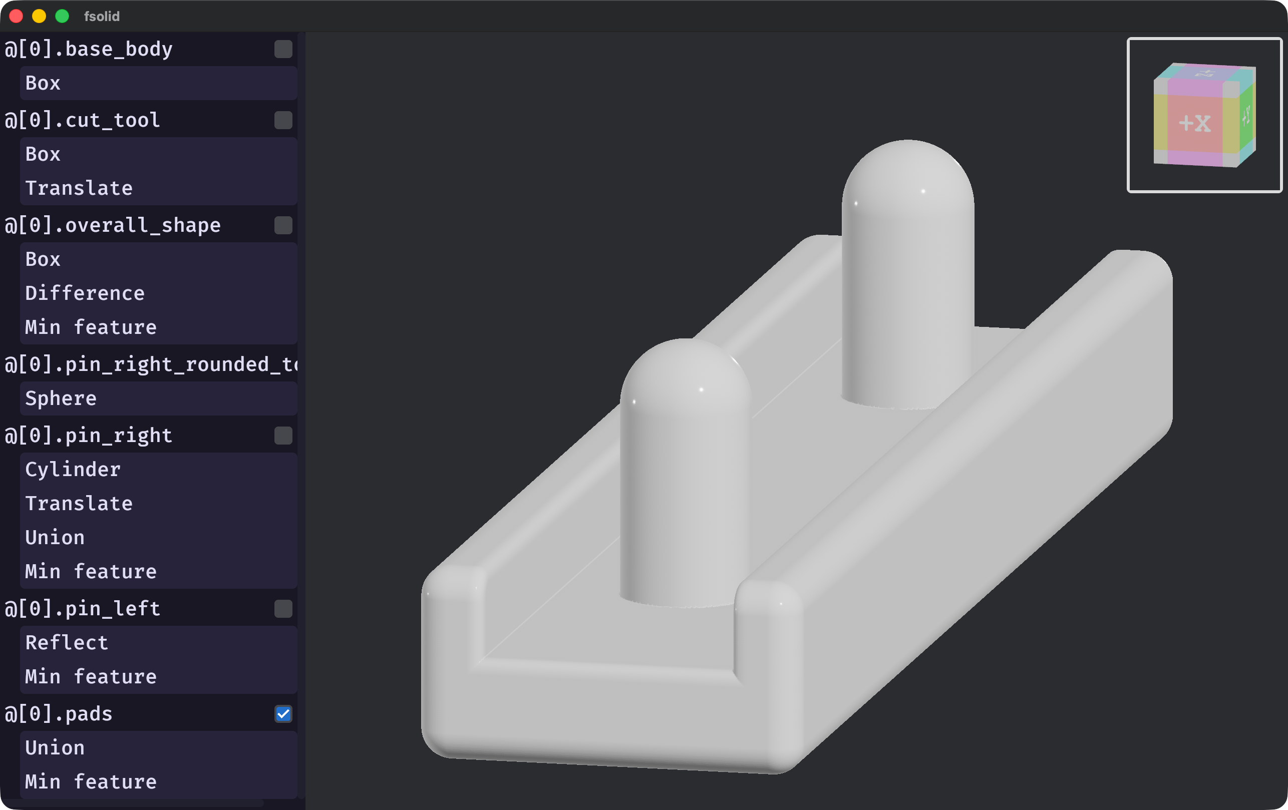
fsolid (v0.6.0).This was my first real experience with CAD, both as a user and as a developer.
This means I’m not a domain-expert; take what I wrote in this article with a grain of salt.
This blog entry is about the tribulations of a feverish desire to render arbitrary implicit surfaces on screen at interactive speed in the context of a mechanical CAD software.
It’s meant as a showcase of this part of my project, documenting why I made certain decision, and maybe sprouting new ideas in someone else’s mind.
Introduction
Before starting our descent into this rabbit-hole, one should empower oneself with the basic understanding of what is
an Implicit Surface (IS) and (Signed) Distance Fields (SDF).
Great explanations exist elsewhere1 2 3; it is encouraged that the uninitiated reader consult them before
diving any further.
In the CAD software I’ve used, which had graphical interfaces, features are added or modified by the user and the viewport reflect those changes.
In some instances, the viewport allows the user to directly drag or scult features using a pointing device.
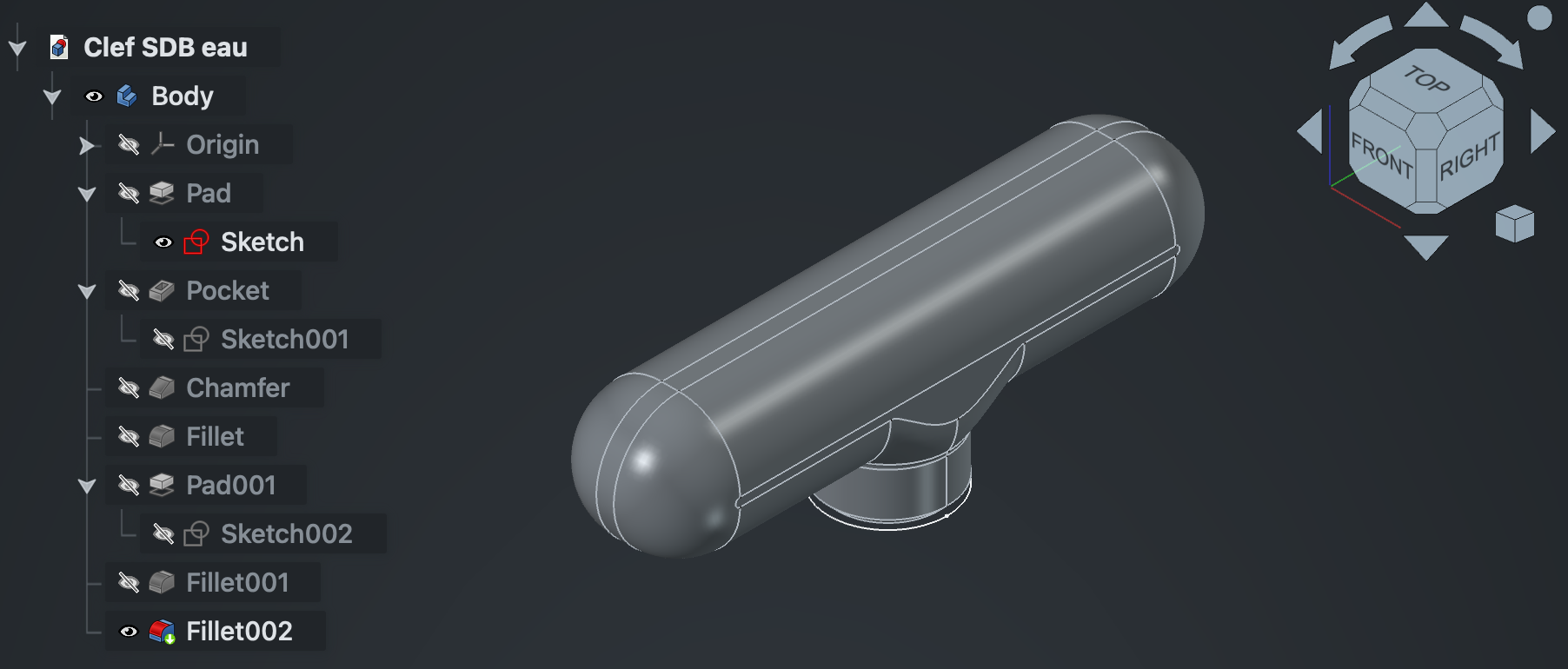
After the modification has been made, the resulting 3D object can be rendered. This include panning, rotating, zooming, or a combinations of those.
Most CAD software use Explicit Surfaces (ES) (e.g., NURBS, Mesh, etc…).
Most processes downstream of authoring (e.g., visualization, CAM, FEM, etc…) require some form of ES.
Rendering is usually done by converting the ES to a triangle mesh, as GPUs are very much optimized for this.
On the other hand, IS describes a volume, discretizing the isosurface is expensive.
While algorithm exists to convert IS to a triangle mesh4 5, they can be slow, produce very large meshes, and may require a complete recomputation on partial changes.
They are necessary to export to a triangle mesh for downstream usage, but other strategies may be used for visualization6.
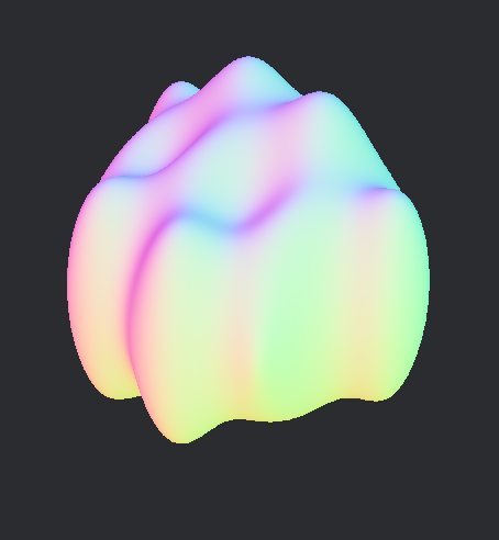
fsolid (commit 96ad96646e)).For this project, I wanted to try and make an IS visualization that would scale with shape complexity, screen resolution and which would happen in two phases.
A loading phase, happening on the CPU, then a rendering phase, which would happen each frame on the GPU.
The priority is smooth movement over up-to-date rendering. This means that while an IS is still loading, a previous version may be showed on screen.
Optionally, I wanted that the rendering be some kind of Montecarlo process, enhancing responsiveness at the cost of quality, while the discretizing is happening.
The technique described today will focus on a two-phase rendering: discretizing and tracing.
It discretize the IS in a data-structure which will be traceable by the GPU.
This project uses fidget, an excellent closed-form IS library.
The rendering is done via wgpu and bevy.
Sampling the void
Bounding volume
An IS only describes a volume.
We don’t yet know where that volume is in space.
For that, we’ll use a bounding volume,
an Axis-Aligned Bounding Box (AABB).
The AABB does multiple things for us.
- It limits the space we need to consider.
- It gives us a simple and efficient way to do ray-slab intersection test, which will come in handy.
- It will allows for fast z-ordering of non-overlapping regions.
AABB can be computed from common IS7 and boolean operations can combine multiple AABB into the resulting IS’s AABB.
For unbounded IS, one should be able to provide an AABB to limit the IS to a certain domain.
Using and representing voxels
The IS’s AABB is rectangular cuboid. We can trivially divide it into a subset of cubic voxel.
Because the isosurface is just a small portion of the AABB’s space, we’ll use a data structure which encode sparse data efficiently:
a variant of Sparse Voxel Octree (SVO).
This variant is a sparse voxel tree, which is sometimes named contree.
Each level of the contree divides its space by 4 on each axis, dividing its space into 64 voxels.
Loading a contree
The algorithm to load the contree need a way to sample the IS in 3 ways:

Interval: this is done to prune large regions of space as entirely empty, full or ambiguous. This testing is conservative; regions which are in fact truly empty might appear as ambiguous in the interval testing.
Regions that are entirely contained by the IS may also be pruned.

Distance: this will be useful to detect where the isosurface is and how far it is from the sampled points.
fidget allows sampling multiple points at once, to amortize the overhead of running the execution tape.

Gradient: this yields a gradient of the IS at a given point, which we’ll use as a surface normal“.
It’s also possible to get a surface normal using the distance sampling (i.e., using forward or central differences).
fidget provides these 3 features.
It also provides great performance1—I encourage readers to check it out
(e.g., JIT, tape simplification, heap buffer re-use, etc…).
Stop condition
When loading a contree, one needs to know when to stop subdividing any further.
We can calculate a stop condition by knowing the minimum feature size we’d like to be able to detect. From the AABB size and this minimum
feature size, we can calculate a contree depth we should be reaching.
Recursive interval testing
We recursively divide the space we consider into 64 voxels, performing interval tests and only consider the voxels which have an ambiguous interval result.
The recursion stops when we get at the desired depth.
Detecting isosurface crossing
Upon reaching the desired subdivision level, we can start sampling distances to find out the voxels which contain the isosurface.
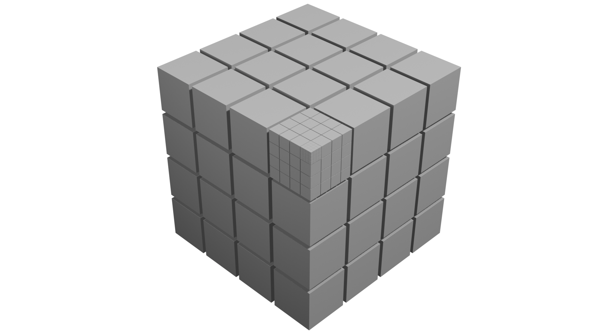
For each leaf node, we want to sample the 64 voxels, but are interested in the vertices of the voxels rather than their center.
Effectively, we’re interested in the dual graph of the voxel grid.
Each voxel has 8 vertices, times 64, naively, that’s 512 points we need to sample.
However, the voxels are tightly packed in our representation and they share vertices with their neighbors.
We can count 5 unique vertices in a row or column of voxels. .
To amortize the execution overhead, we can sample those 125 points in single tape execution.

Populated voxel are highlighted.
The vertices we’re interesting in for our contree are in blue.
We can then iterate over the 64 voxels, checking if there is a sign change in the distance from one of their 8 vertices.
Using this, we create a list of populated voxels and also keep the sampled distances for the vertices of the populated voxels.
Once the 64 voxels are checked, we calculate the gradient for each of the vertices that we kept around.
Summary
We now have all the information we need to load a contree:
- Which voxels are populated, their position and depth in our contree.
- A distance to the surface for each of their vertices.
- A gradient for each of their vertices.
The next step is to serialize this structure so it’s usable.
Serializing the contree
I chose to have a serialization format which I could build while loading the contree.
For simplicity, I also wanted to have the same representation on the CPU and GPU side.
contrees basics
Each node of the contree can address 64 voxels, its population mask fitting exactly 64-bits.
Additionally, a header is necessary to hold some metadata about the node. The header needs to encode a flag
to differentiate non-leaf from leaf nodes and a pointer.
For non-leaf nodes, the flag is unset.
The semantic of the pointer change depending on the type of node.
The childmask only encode the population of the voxel, associated data are necessary and stored elsewhere.
The contree will be encoded by the CPU into the main memory and will be uploaded to the GPU for tracing.
GPUs have fairly strict requirements and limitations in terms of memory alignments, maximum buffer size, etc…
To account for this, the contree will be built in a Structure of Arrays (SoA) style, using 32-bits pointers
to address those (64-bits support is uncommon in GPUs).
Array of Structures of Arrays
The contree will need to be uploaded and consumed by the GPU. To make accessing efficient and cache-friendly we can make it into an Array of Structures of Arrays (AoSoA).
To do that, we’ll make heavy use of 32-bit pointers into our contree, into various arrays.
The contree is split into 4 buffers:
Nodes
They are the leaf and non-leaf nodes of the contree, they were already mentionned in a previous section.

They may look something like this in code:
struct Node {
   header: u32,
   pop_mask: u64
}
This structure spans 12 bytes.
Due to alignment, it may span 16 bytes instead (c.f. rust alignment of primitive types).
Alignment is platform specific, so YMMV.
This is kept as a u64 for now as we benefit from functions exposed by the u64 type (e.g., u64::count_ones). It would be interesting
to measure the performance impact of storing it as two u32 instead, as the memory footprint for this buffer would decrease by 25%.
wgpu doesn’t support 64-bits types by default, to upload this structure to the GPU, we can convert it to 3 u32 instead.
struct GPUNode {
   header: u32,
   pop_mask_hi: u32,
   pop_mask_low: u32,
}
This new form is compatible with the alignment that wgpu requires, as u32 types are aligned on a 4-bytes boundary8.
Leaf nodes
For leaf nodes, the flag is set in the header.
The pointer is an absolute offset to the first leaf indirection in the corresponding buffer (c.f. the next section on the topic).
The leaf indirections are placed in their population mask order, in the leaf indirection buffer.
Non-leaf nodes
For non-leaf nodes, the flag is unset in the header.
The pointer is an absolute offset to the first child in the node buffer.

Each set bit in the population mask represent a populated child.
The children are densely packed in their population mask order, in the node buffer.

Leaf indirections
The leaf indirections are made up of two offsets into the two remaining buffers:
- An absolute offset into the leaf data buffer.
- A partial offset into the vertex data buffer (See the leaf data section to get the absolute offset).
Both in rust and in wgsl, this structure looks like this:
struct LeafIndirection {
   leaf_data_offset: u32,
   vertex_buffer_offset: u32
}
This structure should have no padding due to alignment and spans 8 bytes per entry.

The pointer of leaf nodes is the absolute offset into the leaf indirection buffer.
Leaf data
The leaf data buffer contains 8 partial offsets into the vertex data buffer, one for each of the voxel’s vertices.
This structure is the same both in the CPU and GPU world, having no padding due to alignment and spanning 64 bytes.
struct LeafData  {
   c000: u8,
   c001: u8,
   c010: u8,
   c011: u8,
   c100: u8,
   c101: u8,
   c110: u8,
   c111: u8,
}
Each partial offset is in the range (the maximum number of vertices per node).

Using the leaf data offset from the leaf indirection buffer, one can find the offset into the leaf data buffer
where to start reading for this leaf node.
For each leaf node with populated children, one can expect to find LeafData entries at the leaf data offset.
Because we deduplicated shared vertices when loading the contree, some offsets may be shared by multiple vertices.
Vertex data
Each vertex data contains a distance and normal.
This structure has no padding due to alignment and spans 16 bytes.
struct VertexData {
   normals: vec3f,
   distance: f32,
}
By adding together the vertex buffer offset, from the leaf indirection buffer and the offset for a given vertex in the leaf data buffer, we get the absolute offset into the vertex data buffer.
Space addressing
At each level of the contree, the voxels can be addressed using a Morton Code encoding.
pub struct MortonCode(pub u8);

impl MortonCode {
    pub const fn new(x: u8, y: u8, z: u8) -> Self {
        debug_assert!(x < 4);
        debug_assert!(y < 4);
        debug_assert!(z < 4);

        Self(z << 4 | y << 2 | x)
    }
The value of the MortonCode is in the range .
The MortonCode is used to set the population bit in the node’s childmask.
By having a list of MortonCode of D element, where D is the depth of the contree, one can access a particular voxel.
I’m calling such a list a Morton Path.
To get the space coordinate at a given voxel, one need to use the bounding box of the contree.
You can trivally reverse the Morton Code encoding to get back the x, y and z components.
From these you can calculate an offset from the bounding box minimum.
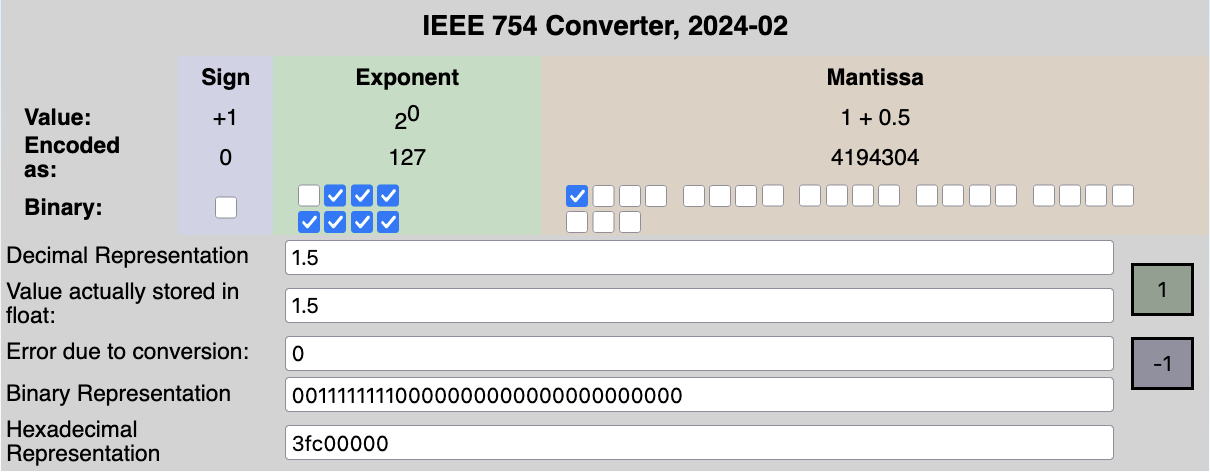
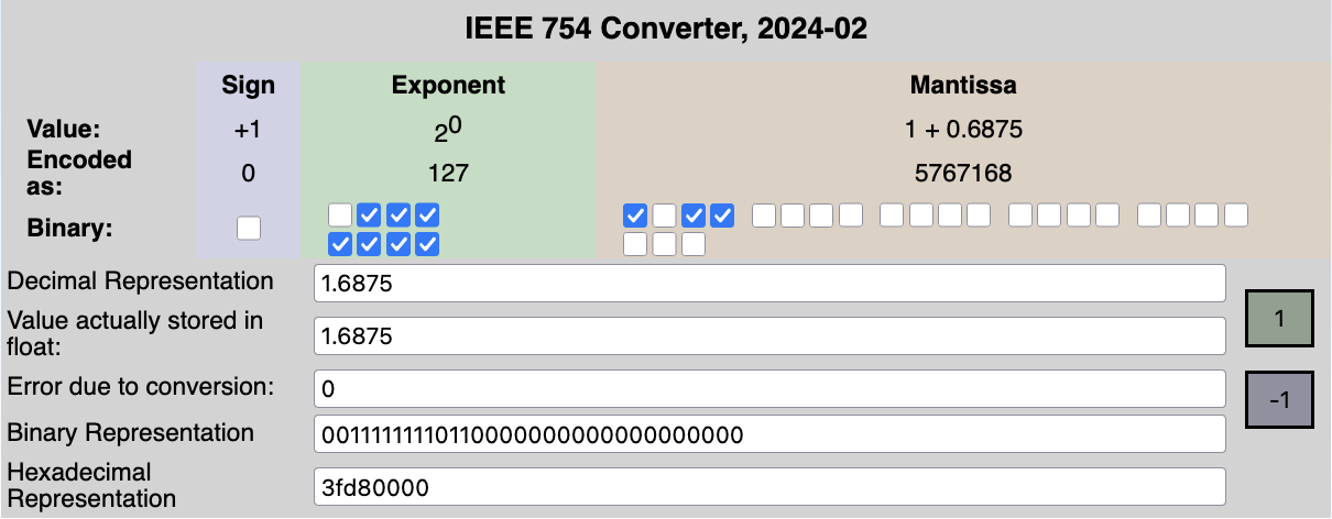
This encoding can also be leveraged from the way IEEE754 floats are represented.

by fresheneesz at the english wikipedia project, cc by-sa 3.0, link
In the exclusive range , the 23 least importants bits of a 32-bits floats can be used to encode a Morton Path.
Splitting those 23 bits in chunks of 2 gives us 11 Morton Path entries and 1 bit to spare.

This idea is quite elegant, though not my own9.
This technique may be used to convert voxel positions in the contree to and from floats.
Maximum depth
As we saw in the Space addressing section, we can only address contree with a depth of 11.
A tree spanning a region of size would be able represent, at best, a voxel of size .
Tile Grid
Having a shorter forest instead of a tall tree
contrees have their challenges.
Even if the loading of the contree could be done in parallel, in my experience, it was much slower than a single-threaded process due to poor cache-locality and massive parallelism overhead.
The memory footprint of contrees also scales with depth, each additional layer of contrees requiring more intermediate nodes.
This is important for tracing, as memory streaming can easily be a bottleneck in GPU applications.
Modifying a contree is a non-trivial operation using the current in-memory and serialization format.
Optimizing for modification could mean changing this format and requiring an actual serialization process.
It’s unclear if the faster modification time would offset the new serialization step and if this change would be a net positive in terms of execution time and memory footprint.
However, some of those challenges can be addressed by adding another layer of indirections: tiles.
Using tiles to discretize our IS means using more than a single contree, by tiling our IS’s region beforehand, and having at most one contree per tile.
Loading a tile grid
Instead of discretizing the IS’s space into one contree, we can first
divide this space into a grid of tiles (rounded-up), stored in a 3 dimensional array.
Each tile is a cubic region of space that is either empty or contains a contree.
For each of the tiles, we can sample the IS interval in the region to determine if the isosurface might be inside. Empty tiles are ignored and a contree is loaded for ambiguous tiles.
This operation can be nicely parallelized.
I used a benchmark that discretizes a region of units across.
Using 1 tiles with a contree depth of 4 is equivalent to using 16 tiles per axis with a contree depth of 2.
Note: a contree of depth 0 still divides by 4 on each axis, each level divides by

Median time: 48.38ms.

Median time: 1.21ms.
Of course, it is fairly obvious that parallelizing such process will reduce the overall runtime by quite a bit.
Serializing a tile grid
Serialization of the tile grid is a very similar to the technique used for the contrees, we just add one more layer of indirection using two new buffers: tile and the tile indirection buffers.
The tile buffer is a list of u32.
A special value of u32::MAX signals that the tile is empty, otherwise, the value is a pointer into the tile indirection buffer.

The absolute offsets we used in the contrees are now partial offsets.
One need to add the tile indirection offsets to get the starting index for a given tile.
Choosing the right tile size
Choosing the tile size is a game of balance between the size of the 3D array that will contain the tiles, the depth of the contrees and the minimum feature that will be discretizable.
Also notably, the number of tiles will directly affect the number of tasks to parallelize. Having too much tiles causing the overhead of the parallelization to be greater per task.
On the other hand, having too few tiles causes poor distribution of load and possibly deeper contrees.
From my crude benchmarks, an empirical maximum number of tiles is .
Looking at the benchmarks, we can see the scaling the number of tasks to parallelize to the number of tiles to discretize quickly has its limit:
Median time: 1.21ms.

Median time: 53.47ms.
The benchmark discretize a region of units across.
Using 16 tiles per axis with a contree depth of 2 is equivalent to using 64 tiles per axis with a contree depth of 1.
Even though the resolution produced by those benchmarks is the same, there is a increase in mean runtime when using the larger number of tiles.
This is mainly due to the number of tasks to parallelize, the overhead that goes with it, and the added memory pressure of having to manage a larger 3D array for the tiles.
Tracing the void
Now that we’ve sampled the void, we should briefly talk about how to use this with GPU to show some nice images.
This section is intentionally brief, as it relies on well-known algorithms that are better explained elsewhere9.
For this project, I’ve been using the bevy game engine.
The plan is:
- Upload the IS and camera-related data to the GPU.
- Spawn a proxy mesh for each IS in the scene. By using this proxy mesh, I can benefit from the CPU culling built into
bevy. - For each IS in view, allocate a texture (depth and normal).
- If the IS has changed, or if the camera has moved or if it the texture has never been rendered, schedule a compute shader to trace the IS and populate the texture.
- Perform a depth pre-pass.
- Using the texture and a fragment shader, add Physically Based Rendering to the populated pixels.
Uploading data to the GPU
The data structure we’ve been building (c.f. Serializing the tile grid) can be uploaded to some GPU buffers nearly as-is.
Some additional data should also be uploaded in uniforms buffers, such as:
- Camera matrixes.
- IS metadata (transform, AABB).
- tile grid metadata (tile size, grid size).
An additionnal optimization is to limit the bytes transferred per frame to avoid stuttering and spread uploading over multiple frames.
Compute shader ray-marching
To rasterize the texture we’ve allocated, we can use a compute shader, which has finer control over the parallelism we use over fragment shaders.
We can divide the texture into a grid of texture tiles and dispatch an appropriate amount of workgroups.
This compute shader shoot a conceptual ray going from the camera, into the scene.
If the ray intersects the IS’s AABB, we can start marching the tiles.
If the ray misses the AABB, we can exit early.
Marching the tiles
After the ray has intersected the AABB, we can figure out in which tile the ray currently is.
Using the Digital Differential Analyzer (DDA) algorithm, we can step through the tile grid until we hit a populated tile or exit the grid.
Upon hitting a populated tile, we march the inner contree.
The range of steps is where number of tiles per axis.
Marching the contrees
Marching the contree uses a recursive version of the DDA algorithm, which is really best described in dubiousconst282’s blog9.
When the ray intersects with a populated voxel of a leaf node in the contree, we can use the associated data to gather the 8 distances and normals for this voxel’s vertices.
We can perform a trilinear interpolation of the distance and normal from the ray-voxel intersection at this point.
The range of steps is .
Combined marching
If the ray misses the inner contree populated voxels, we continue stepping into the tile grid normally.
The range of steps is where number of tiles per axis.
If the ray doesn’t intersect a populated voxel and exit the bounding volume, we can exit the shader early.
Alpha mode
When rendering our proxy mesh, we have to choose the correct alpha mode to render in.
To render an opaque IS, we need to use the Mask mode.
That is because we want some transparency, so that rays that do not intersect with the IS do not participate in the final rendering.
This mode is also cheaper to use that other mode allowing some form of transparency.
For transparent IS, one can use any of the transparent mode (e.g., Blend, Premultiplied, Add, or Multiply).
Depth prepass
Integrating this rendering process with a depth prepass allows to render multiple IS mixed with normal meshes and have them render at the correct depth.
This integration happens in 2 steps:
- During a depth prepass, a special fragment shader will report the depth of the populated pixels. When multiple IS report their depth, the one closer to the camera is saved used.
- During the main pass fragment shader, the fragment depth is compared with the depth gathered during the prepass.
If the current depth is further away from the camera than the depth prepass stored value, the fragment is discarded.
This setup also works for non IS based elements, like a mesh object (i.e. the purple taurus).
Fragment shader
The fragment shader will run on each frame.
It is responsible for reading the texture populated by the compute shader and applying PBR to it.
How fast is it?
Well, I don’t exactly know.
I’m not exactly sure how to benchmark this type of project, other than running an example scene and moving the camera a lot.
So here I am doing exactly that. I disabled VSync so the FPS are not tied to my display’s refresh rate.
Note: the compute shader only runs when the scene changes or when the view changes.
That is why you can see the FPS going higher when there is no movement, compared to when I’m moving the camera.
The prepass and main pass shader run every frame.
The window resolution is 2560x1440, but the texture being rendered are constantly resized as the view change.
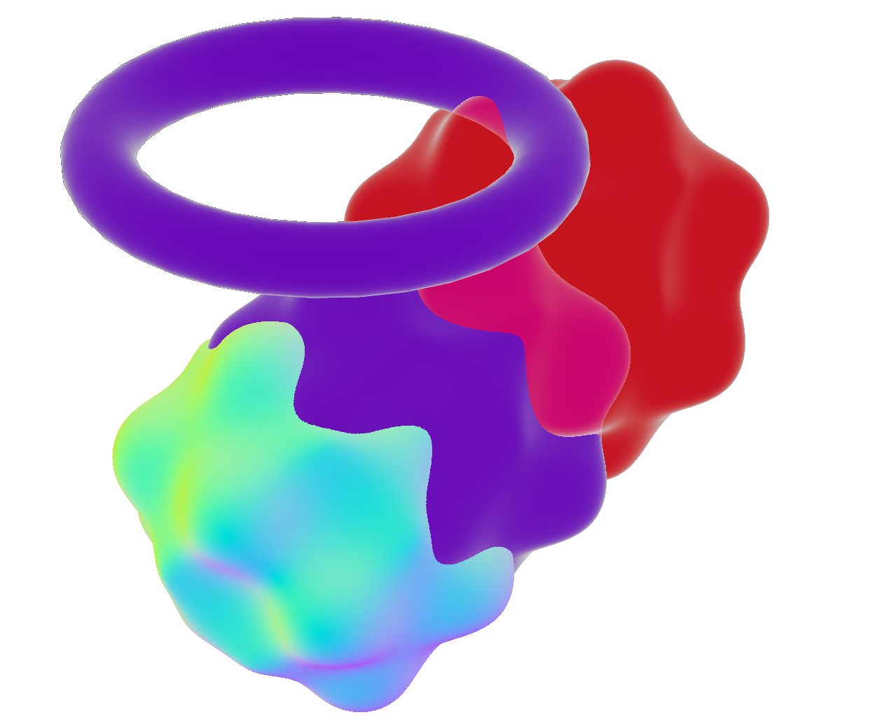
The scene I’m using displays 4 spheres with surface distortions, each with a different rendering mode.
There is a cuboid shape that is also an IS of negligeable size and a mesh-based taurus.
The computer I’m running these benchmarks on is an Apple Mac Book Pro M2 Max (2022) running Mac OS Tahoe 26.3.1.
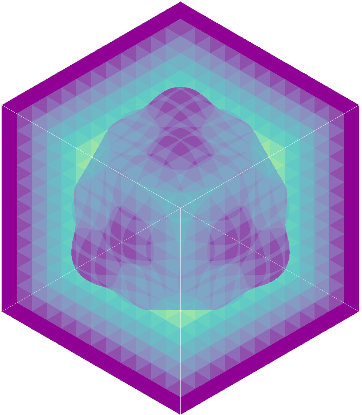
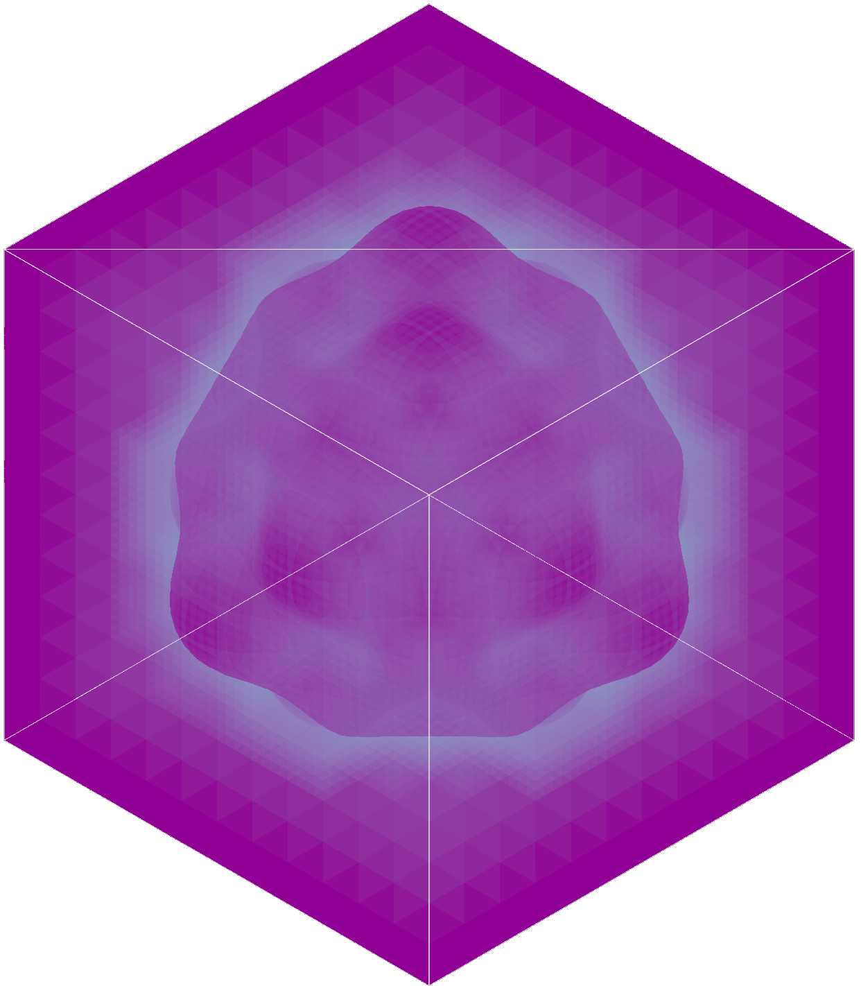
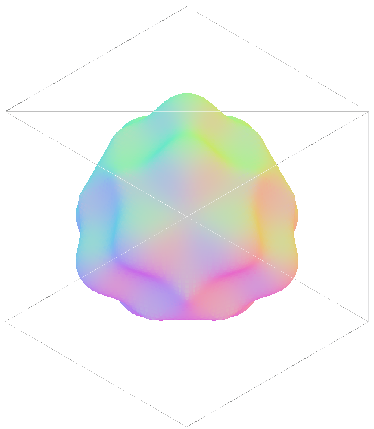
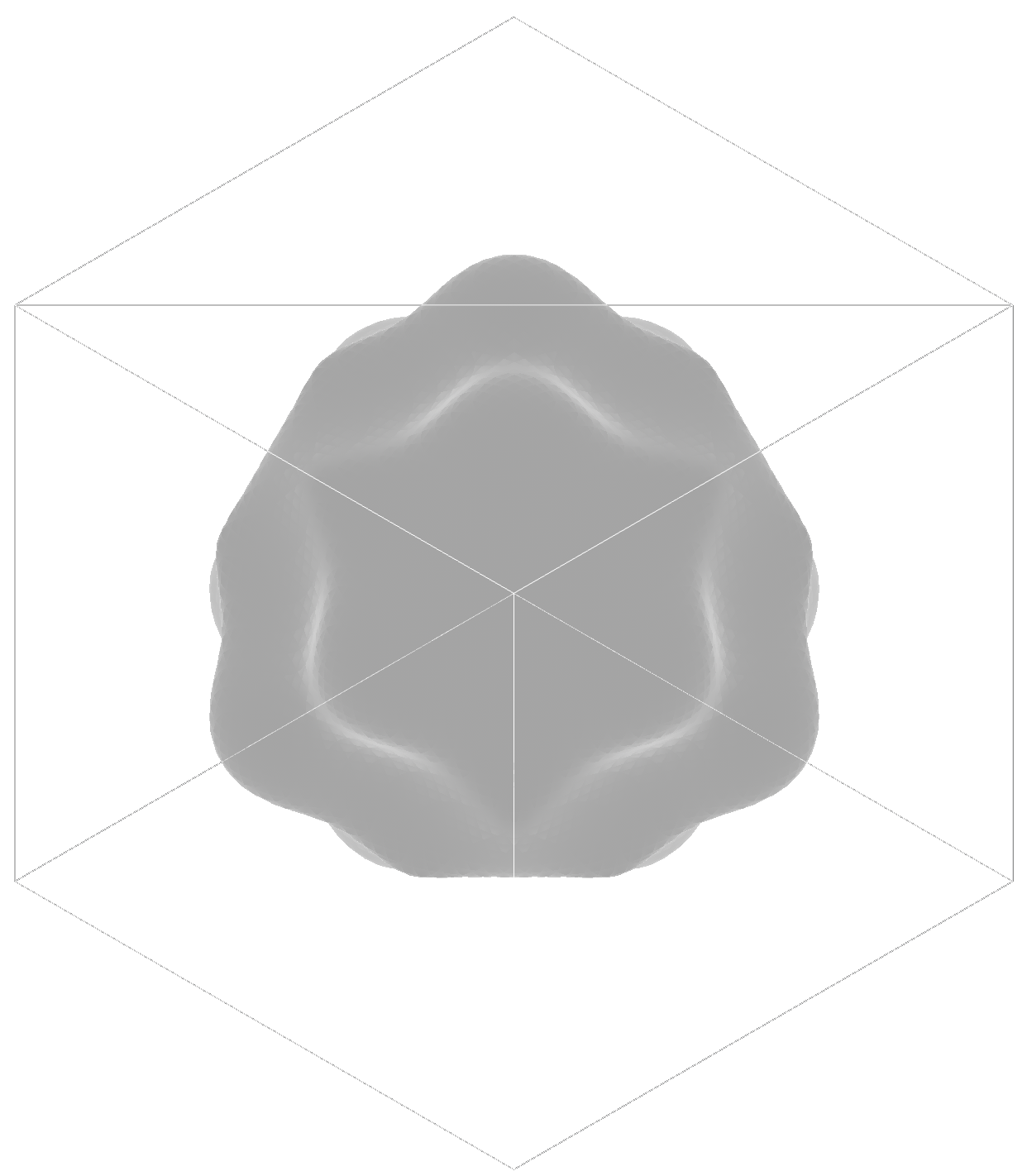
The distorted spheres have a maximum diameter of 11 units. I’ll be modifying the minimum feature size of these spheres to scale up the discretization.
0.1 units minimum-feature size for the distorted spheres.They take up ~4.266 MB of memory.
The movements are smooth (>=60 FPS), even when zoomed-in multiple medium-resolution IS.
The edges where the IS intersects have a few artifacts due to the insufficient resolution in those regions.
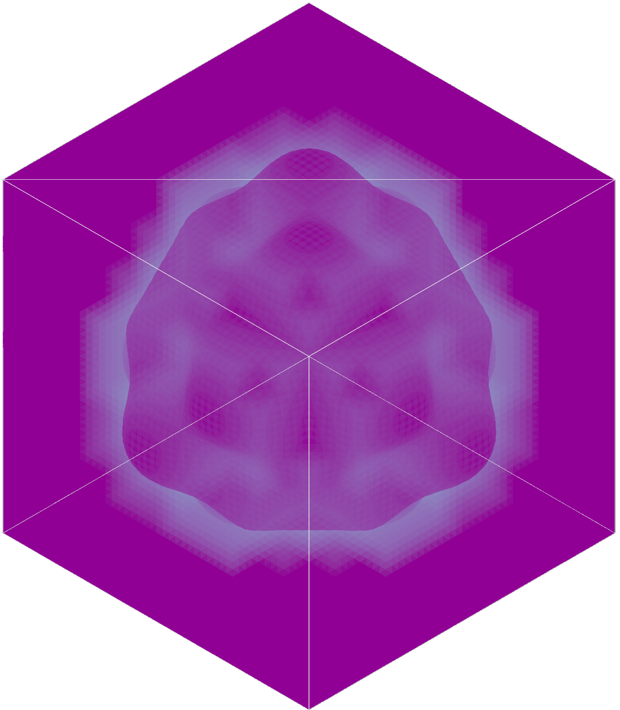
0.01 units minimum-feature size for the distorted spheres.They take up ~470.632 MB of memory.
The movements stay at editable speeds (>=30 FPS), when zoomed-in on high-resolutions IS.
The edges where the IS intersects are now very sharp.
Closing words
This was a fun endeavor, albeit a tad fever-inducing, especially when trying to write long and complex wgpu shaders.
Feel free to browse and judge my woefully undocumented code on the fsolid’s project page, especially the relevant crate bevy_is.
Things to try next (maybe)
Reduce memory footprint
The memory footprint of these structures can get quite high, especially for a constrained environment such as a GPU.
A low-hanging optimization is splitting up the u64 used in the population mask to into 2 u32 to embetter the alignment and the memory usage on the CPU side.
Another, more complex one, would be to transform the Sparse Voxel Tree into a Sparse Voxel Directed Acyclic Graph10.
This could drastically reduce the size some discretized IS would take in memory.
This reduction in size could in turn have a positive effect on the rendering
time by the GPU, as it could mean a better usage of cache and data locality.
Optimize GPU tracing
Of course, the main goal for this would be better user experience, unlocking support for lower power devices and lowering energy consumption.
There are some fairly low-hanging optimizations that are documented9 which I didn’t include, either because of time constraints or because I don’t understand them yet.
Some more complex, such as the beam optimization11.
Better parallelism
Treating the tile grid as a tree of tiles could reduce the parallelism overhead of large and sparse tile grids.
Otherwise, adding some smarter parallelism to the contree’s loading could reduce the number of tiles in the tile grid, whilst keeping the same rendering resolution.
This would also unlock some of the performance benefits (i.e., skipping large empty region in one step) that tracing contree have, but that are minimized by their smaller size in the current rendering.
References
-
Dual Contouring of Hermite Data (2002), Tao Ju, Frank Losasso, Scott Schaefer, Joe Warren Rice University ↩
-
Marching cubes: A high resolution 3D surface construction algorithm (1987), Lorensen, William E. and Cline, Harvey E. ↩
-
Sphere Tracing: A Geometric Method for the Antialiased Ray Tracing of Implicit Surfaces (1995), John Hart ↩
-
A guide to fast voxel ray tracing using sparse 64-trees, dubiousconst282 ↩ ↩2 ↩3 ↩4
-
High resolution sparse voxel DAGs (2013), Kämpe, Viktor and Sintorn, Erik and Assarsson, Ulf ↩